Tim Duff, GA Tech
joint w/ Kathlén Kohn (KTH) Anton Leykin (GT)
& Tomas Pajdla (CIIRC)
SIAM Virtual MDS20 "in Cincinnati"
Session on Algebraic Geometry and Machine learning
Overview
- Background
- Geometry in computer vision
- What is a minimal problem?
- Classifying minimal problems
This work began at ICERM in Fall 2018, along with
Trifocal Relative Pose from Lines at Points (w/ Fabbri, Fan, Regan, ...) Next week at CVPR!
Trifocal Relative Pose from Lines at Points (w/ Fabbri, Fan, Regan, ...) Next week at CVPR!
Numerically stable, relatively fast ($\sim 1$s for $312$ solutions) homotopy continuation solver
Real-time requirement: $<<1$ms...
A long-term challenge relevant to this minisymposium is to assist HC with heuristics obtained by learning
Real-time requirement: $<<1$ms...
A long-term challenge relevant to this minisymposium is to assist HC with heuristics obtained by learning
- What is the right formulation?
- What are the right training data?
- Need to make inference/prediction fast
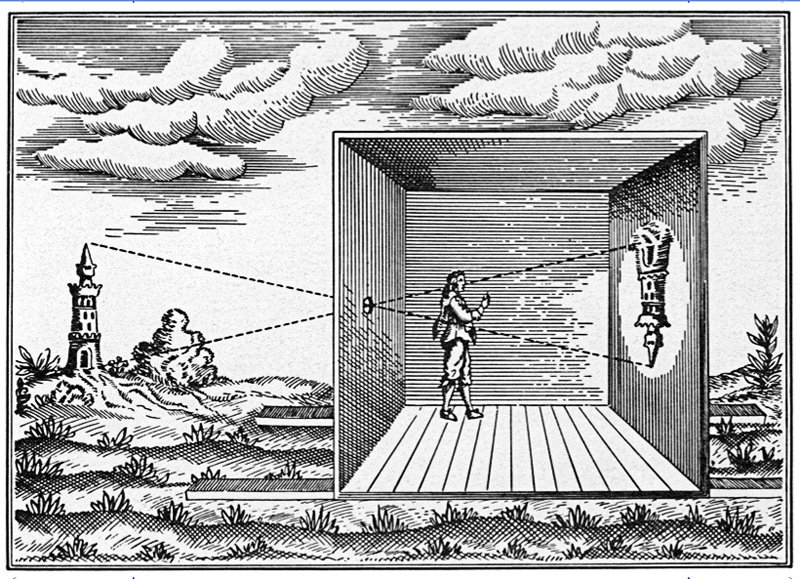
 (Hartley-Zisserman, 00)
Pinhole camera is a projective-linear map:
\[
[X:Y:Z:1] \mapsto [X/Z:Y/Z:1] = [X:Y:Z]\\
\big( \text{ in suitable coordinates with } \, f=1 \big)
\]
Calibrated camera: known internal parameters, like $f$
Measured point correspondences: $x_1, \ldots, x_n, y_1, \ldots , y_n \in \mathbb{P}^2$
Unknown: change of coordinates & $n$ world points
An Efficient Solution to the Five-Point
Relative Pose Problem (Nistér, PAMI 2004)
Implementation: eg. COLMAP (Schönberger, 2019)
(Nistér, PAMI 2004)
Implementation: eg. COLMAP (Schönberger, 2019)
Lines as features?
Part II: Complete visibility
\[\begin{aligned}
\DeclareMathOperator{\SO}{SO}
m = \# \text{ number of views}\\
p = \# \text{ points in each view}\\
l = \# \text{ lines in each view}\\
\mathcal{I} \subset \{ 1, \ldots , p \} \times \{ 1 , \ldots , l \} \text{ --- prescribed incidences}\\
\mathcal{X} = \left\{ (X, L) \in \left( \mathbb{P}^3 \right)^p \times \left( \mathbb{G}_{1,3} \right)^{l} \mid \forall (i,j) \in \mathcal{I}\, \colon X_i \in L_j \right\}\\
\mathcal{C} = \{ \left( [R_1 \mid t_1], \ldots , [R_m | t_m] \right) \mid
R_i R_i^\top = I , \det R_i = 1,
\, \, \, \, \, \, \,
\\
\, \, R_1 = I, \, t_1 = 0, \, t_{2,1} = 1 \} \\
\mathcal{Y} = \left\{ (x, \ell) \in \left(\mathbb{P}^2 \right)^{m\, p} \times \left( \mathbb{G}_{1,2} \right)^{m \, l} \;\middle\vert\;
\, \, \, \, \, \, \, \, \, \, \, \, \, \, \, \, \, \, \, \, \, \, \, \, \, \, \, \, \, \, \, \, \, \, \, \, \, \, \,
\\
\, \, \, \forall \, \, v=1,\ldots,m \, \,
\forall \, \,
(i,j) \in \mathcal{I} \, \, \, \, x_{v, i} \in \ell_{v, j} \right\} \\
\\
\\
\end{aligned}
\]
Old paper: exactly 30 minimal problems in this setting

!!!!!!!!!!!!!
Checking minimality:
\[\begin{aligned}
\\
\\
\\
\\
\\
\\
\\
\\
\text{Sample: } (x,c) \in \mathcal{X} \times \mathcal{C} \\
\textrm{rank } D_{x,c} \Phi (x, c) = \dim \mathcal{Y}?\\
\end{aligned}
\]
Part III: Partial visibility
Motivation:
It is easy to construct infinitely many minimal problems in 3 views.


\[\begin{aligned}
\DeclareMathOperator{\SO}{SO}
\newcommand{\PP}{\mathbb{P}}
\newcommand{\GG}{\mathbb{G}}
\mathcal{X}, \mathcal{C} \text{ --- as before } \\
\mathcal{Y} =\left\{ (x, \ell) \in \left(\PP^2 \right)^{\rho} \times \left( \GG_{1,2} \right)^{\lambda} \mid \\
\begin{array}l
\forall v=1,\ldots,m \;
\forall i \in \mathcal{P}_v \\
\forall j \in \mathcal{L}_v \,
(i,j) \in \mathcal{I}
\Rightarrow
x_{v, i} \in \ell_{v, j}
\end{array}
\right\}
\end{aligned}
\]
$\mathcal{P}_v, \mathcal{L}_v$ record observations in each view $v=1,\ldots , n.$
Subproblems are obtained by deleting corresponding features from 3D and 2D.
Reduction to a subproblem
\[
\begin{aligned}
\mathcal{X} & & \rightarrow & & \mathcal{Y} \\
\downarrow & & & & \downarrow \\
\mathcal{X}' & & \rightarrow & & \mathcal{Y}'
\end{aligned}
\]
Reduced means no nontrivial reductions
Reduction: delete feature correspondences
"Reduction": minimal to camera-minimal


minimal camera-minimal
Applying both reductions and "reductions" yields terminal camera-minimal problems.
$\textrm{PL}_k\textrm{P}$---each line incident to at most $k$ points
Problem hierarchy: \[ \textrm{PL}_0\textrm{P} \subset \textrm{PL}_1\textrm{P} \subset \textrm{PL}_2\textrm{P} \subset \cdots \]
$\text{PL}_0P$s --- "reduced minimal" and
"terminal camera minimal" coincide.
Low-degree $\text{PL}_1 P$s:
end of talk; thank you!
$\text{PL}_0P$s --- "reduced minimal" and
"terminal camera minimal" coincide.
Low-degree $\text{PL}_1 P$s:
Minimal when $2 \times 2 \times n = \underbrace{5}_{t\in \mathbb{P}^2} + 3\times n$
Relative Pose Problem (Nistér, PAMI 2004)
Implementation: eg. COLMAP (Schönberger, 2019)
std::vector<EssentialMatrixFivePointEstimator::M_t&rt
EssentialMatrixFivePointEstimator::Estimate(const std::vector<X_t&rt& points1,
                                            const std::vector<Y_t&rt& points2) {
  CHECK_EQ(points1.size(), points2.size());

  // Step 1: Extraction of the nullspace x, y, z, w.

  Eigen::Matrix<double, Eigen::Dynamic, 9&rt Q(points1.size(), 9);
  for (size_t i = 0; i < points1.size(); ++i) {
    const double x1_0 = points1[i](0);
    const double x1_1 = points1[i](1);
    const double x2_0 = points2[i](0);
    const double x2_1 = points2[i](1);
    Q(i, 0) = x1_0 * x2_0;
    Q(i, 1) = x1_1 * x2_0;
    Q(i, 2) = x2_0;
    Q(i, 3) = x1_0 * x2_1;
    Q(i, 4) = x1_1 * x2_1;
    Q(i, 5) = x2_1;
    Q(i, 6) = x1_0;
    Q(i, 7) = x1_1;
    Q(i, 8) = 1;
  }

  // Step 2: Extract the 4 Eigen vectors corresponding to the smallest singular values.
  const Eigen::JacobiSVD<Eigen::Matrix<double, Eigen::Dynamic, 9&rt&rt svd(
      Q, Eigen::ComputeFullV);
  const Eigen::Matrix<double, 9, 4&rt E = svd.matrixV().block<9, 4&rt(0, 5);

  // Step 3: Gauss-Jordan elimination with partial pivoting on A.

  Eigen::Matrix<double, 10, 20&rt A;
#include "estimators/essential_matrix_poly.h"
  Eigen::Matrix<double, 10, 10&rt AA =
      A.block<10, 10&rt(0, 0).partialPivLu().solve(A.block<10, 10&rt(0, 10));

// Step 4: Expansion of the determinant polynomial of the 3x3 polynomial
  //         matrix B to obtain the tenth degree polynomial.

  Eigen::Matrix<double, 13, 3> B;
  for (size_t i = 0; i < 3; ++i) {
    B(0, i) = 0;
    B(4, i) = 0;
    B(8, i) = 0;
    B.block<3, 1&rt(1, i) = AA.block<1, 3&rt(i * 2 + 4, 0);
    B.block<3, 1&rt(5, i) = AA.block<1, 3&rt(i * 2 + 4, 3);
    B.block<4, 1&rt(9, i) = AA.block<1, 4&rt(i * 2 + 4, 6);
    B.block<3, 1&rt(0, i) -= AA.block<1, 3&rt(i * 2 + 5, 0);
    B.block<3, 1&rt(4, i) -= AA.block<1, 3&rt(i * 2 + 5, 3);
    B.block<4, 1&rt(8, i) -= AA.block<1, 4&rt(i * 2 + 5, 6);
  }

  // Step 5: Extraction of roots from the degree 10 polynomial.
  Eigen::Matrix<double, 11, 1> coeffs;
#include "estimators/essential_matrix_coeffs.h"

  Eigen::VectorXd roots_real;
  Eigen::VectorXd roots_imag;
  if (!FindPolynomialRootsCompanionMatrix(coeffs, &roots_real, &roots_imag)) {
    return {};
  }

  std::vector<M_t&rt models;
  models.reserve(roots_real.size());

  for (Eigen::VectorXd::Index i = 0; i < roots_imag.size(); ++i) {
    const double kMaxRootImag = 1e-10;
    if (std::abs(roots_imag(i)) &rt kMaxRootImag) {
      continue;
    }


    const double z1 = roots_real(i);
    const double z2 = z1 * z1;
    const double z3 = z2 * z1;
    const double z4 = z3 * z1;

    Eigen::Matrix3d Bz;
    for (size_t j = 0; j < 3; ++j) {
      Bz(j, 0) = B(0, j) * z3 + B(1, j) * z2 + B(2, j) * z1 + B(3, j);
      Bz(j, 1) = B(4, j) * z3 + B(5, j) * z2 + B(6, j) * z1 + B(7, j);
      Bz(j, 2) = B(8, j) * z4 + B(9, j) * z3 + B(10, j) * z2 + B(11, j) * z1 +
                 B(12, j);
    }

    const Eigen::JacobiSVD<Eigen::Matrix3d&rt svd(Bz, Eigen::ComputeFullV);
    const Eigen::Vector3d X = svd.matrixV().block<3, 1&rt(0, 2);

    const double kMaxX3 = 1e-10;
    if (std::abs(X(2)) < kMaxX3) {
      continue;
    }

    Eigen::MatrixXd essential_vec = E.col(0) * (X(0) / X(2)) +
                                    E.col(1) * (X(1) / X(2)) + E.col(2) * z1 +
                                    E.col(3);
    essential_vec /= essential_vec.norm();

    const Eigen::Matrix3d essential_matrix =
        Eigen::Map<Eigen::Matrix<double, 3, 3, Eigen::RowMajor&rt&rt(
            essential_vec.data());
    models.push_back(essential_matrix);
  }

  return models;
}
5-point solvers
An Efficient Solution to the Five-Point Relative Pose Problem(Nistér, PAMI 2004)
Implementation: eg. COLMAP (Schönberger, 2019)
std::vector<EssentialMatrixFivePointEstimator::M_t&rt
EssentialMatrixFivePointEstimator::Estimate(const std::vector<X_t&rt& points1,
                                            const std::vector<Y_t&rt& points2) {
  CHECK_EQ(points1.size(), points2.size());

  // Step 1: Extraction of the nullspace x, y, z, w.

  Eigen::Matrix<double, Eigen::Dynamic, 9&rt Q(points1.size(), 9);
  for (size_t i = 0; i < points1.size(); ++i) {
    const double x1_0 = points1[i](0);
    const double x1_1 = points1[i](1);
    const double x2_0 = points2[i](0);
    const double x2_1 = points2[i](1);
    Q(i, 0) = x1_0 * x2_0;
    Q(i, 1) = x1_1 * x2_0;
    Q(i, 2) = x2_0;
    Q(i, 3) = x1_0 * x2_1;
    Q(i, 4) = x1_1 * x2_1;
    Q(i, 5) = x2_1;
    Q(i, 6) = x1_0;
    Q(i, 7) = x1_1;
    Q(i, 8) = 1;
  }

  // Step 2: Extract the 4 Eigen vectors corresponding to the smallest singular values.
  const Eigen::JacobiSVD<Eigen::Matrix<double, Eigen::Dynamic, 9&rt&rt svd(
      Q, Eigen::ComputeFullV);
  const Eigen::Matrix<double, 9, 4&rt E = svd.matrixV().block<9, 4&rt(0, 5);

  // Step 3: Gauss-Jordan elimination with partial pivoting on A.

  Eigen::Matrix<double, 10, 20&rt A;
#include "estimators/essential_matrix_poly.h"
  Eigen::Matrix<double, 10, 10&rt AA =
      A.block<10, 10&rt(0, 0).partialPivLu().solve(A.block<10, 10&rt(0, 10));

// Step 4: Expansion of the determinant polynomial of the 3x3 polynomial
  //         matrix B to obtain the tenth degree polynomial.

  Eigen::Matrix<double, 13, 3> B;
  for (size_t i = 0; i < 3; ++i) {
    B(0, i) = 0;
    B(4, i) = 0;
    B(8, i) = 0;
    B.block<3, 1&rt(1, i) = AA.block<1, 3&rt(i * 2 + 4, 0);
    B.block<3, 1&rt(5, i) = AA.block<1, 3&rt(i * 2 + 4, 3);
    B.block<4, 1&rt(9, i) = AA.block<1, 4&rt(i * 2 + 4, 6);
    B.block<3, 1&rt(0, i) -= AA.block<1, 3&rt(i * 2 + 5, 0);
    B.block<3, 1&rt(4, i) -= AA.block<1, 3&rt(i * 2 + 5, 3);
    B.block<4, 1&rt(8, i) -= AA.block<1, 4&rt(i * 2 + 5, 6);
  }

  // Step 5: Extraction of roots from the degree 10 polynomial.
  Eigen::Matrix<double, 11, 1> coeffs;
#include "estimators/essential_matrix_coeffs.h"

  Eigen::VectorXd roots_real;
  Eigen::VectorXd roots_imag;
  if (!FindPolynomialRootsCompanionMatrix(coeffs, &roots_real, &roots_imag)) {
    return {};
  }

  std::vector<M_t&rt models;
  models.reserve(roots_real.size());

  for (Eigen::VectorXd::Index i = 0; i < roots_imag.size(); ++i) {
    const double kMaxRootImag = 1e-10;
    if (std::abs(roots_imag(i)) &rt kMaxRootImag) {
      continue;
    }


    const double z1 = roots_real(i);
    const double z2 = z1 * z1;
    const double z3 = z2 * z1;
    const double z4 = z3 * z1;

    Eigen::Matrix3d Bz;
    for (size_t j = 0; j < 3; ++j) {
      Bz(j, 0) = B(0, j) * z3 + B(1, j) * z2 + B(2, j) * z1 + B(3, j);
      Bz(j, 1) = B(4, j) * z3 + B(5, j) * z2 + B(6, j) * z1 + B(7, j);
      Bz(j, 2) = B(8, j) * z4 + B(9, j) * z3 + B(10, j) * z2 + B(11, j) * z1 +
                 B(12, j);
    }

    const Eigen::JacobiSVD<Eigen::Matrix3d&rt svd(Bz, Eigen::ComputeFullV);
    const Eigen::Vector3d X = svd.matrixV().block<3, 1&rt(0, 2);

    const double kMaxX3 = 1e-10;
    if (std::abs(X(2)) < kMaxX3) {
      continue;
    }

    Eigen::MatrixXd essential_vec = E.col(0) * (X(0) / X(2)) +
                                    E.col(1) * (X(1) / X(2)) + E.col(2) * z1 +
                                    E.col(3);
    essential_vec /= essential_vec.norm();

    const Eigen::Matrix3d essential_matrix =
        Eigen::Map<Eigen::Matrix<double, 3, 3, Eigen::RowMajor&rt&rt(
            essential_vec.data());
    models.push_back(essential_matrix);
  }

  return models;
}
Driving questions:
- What role can algebraic geometry play?
- How to do computations?
$\mathbb{G}_{k,n} = $ Grassmannian of $k$-planes in $\mathbb{P}^n$
$\dim \mathbb{G}_{1,3} = 4$
$\dim \mathbb{G}_{1,2} = 2$
$\dim \mathbb{G}_{1,2} = 2$
$\Rightarrow $ correspondence of $\ge 3$ lines needed to constrain cameras
\[
\Phi : \mathcal{X} \times \mathcal{C} \to \mathcal{Y}
\]
A point-line problem is minimal if $\Phi \left( \mathcal{X} \times \mathcal{C} \right)$ is Zariski-dense in $\mathcal{Y}$ and generic fibers $\Phi^{-1} (x, \ell)$ are finite.
!!!!!!!!!!!!!
Not enough to count dimensions! 
Computing $\Phi^{-1} (x, \ell)$
 (Sturmfels-Miller, 05)
|
|
| Gröbner Bases | Monodromy |
- Missing data / occlusions
- Relaxation of certain correspondence constraints
It is easy to construct infinitely many minimal problems in 3 views.
But aren't these the same?
|
|
|
| reduced | not reduced |
Minimal problems with incidences may "reduce" to camera-minimal problems
minimal camera-minimal
minimal camera-minimal
|
|
|
| reduced | not reduced |
"Reduction": minimal to camera-minimal
minimal camera-minimal
Applying both reductions and "reductions" yields terminal camera-minimal problems.
Theorem (new paper)
There are 74,575 terminal camera-minimal problems in 3 views where every line is incident to at most one point.Problem hierarchy: \[ \textrm{PL}_0\textrm{P} \subset \textrm{PL}_1\textrm{P} \subset \textrm{PL}_2\textrm{P} \subset \cdots \]
Theorem (restated)
There are 74,575 terminal camera-minimal $\text{PL}_1\text{P}$s in 3 views.
Several related results, intricate case analysis.
Main paper: 8 pages, no proofs
Appendix: 12 pages, all proofs
Main paper: 8 pages, no proofs
Appendix: 12 pages, all proofs
"terminal camera minimal" coincide.
| deg | 64 | 80 | 144 | 160 | 216 | 224 | 240 | 256 | 264 | 272 | 288 | freq | 13 | 9 | 3 | 547 | 7 | 2 | 159 | 2 | 2 | 11 | 4 |
"terminal camera minimal" coincide.
| deg | 64 | 80 | 144 | 160 | 216 | 224 | 240 | 256 | 264 | 272 | 288 | freq | 13 | 9 | 3 | 547 | 7 | 2 | 159 | 2 | 2 | 11 | 4 |