Math 4120: Graph Theory and Combinatorics

1. Basic Definitions

The Definition of a Graph

A graph $ G $ consists of a vertex set $ V(G) $, whose elements are called vertices and an edge set $ E(G) $, where elements in $ E(G) $ are unordered pairs of vertices. The elements of $E(G)$ are called edges.

Remarks: Recall that an unordered pair is just any two-element set $\{ u , v \}$, where $u\ne v.$ For brevity, we often write such an edge more simply as $ uv $. In various contexts, it is common to denote an edge by the ordered pair $ (u,v) $. This leads to an alternative definition of a graph, equivalent to ours, as a relation on the vertex set $V(G)$ that is both symmetric (meaning that $ (u,v) $ is an edge if and only if $ (v,u) $ is an edge) and irreflexive (meaning that $ (u,u) $ is never an edge.)

Example 1:

The picture shown above is a visual representation of a graph with the $6$ vertices and $8$ edges given below. $ V(G) = \{1, 2, 3, 4, 5, 6\} $
$ E(G) = \{12, 13, 23, 34, 36, 46, 45, 56\} $.

Neighborhood and Degree

For any edge $ uv \in E(G) $, the vertices $ u, v \in V(G) $ are said to be adjacent and/or neighbors in $ G $. The vertices $ u, v $ are called the ends of the edge $ uv $, and any edge is said to be incident at either of its ends.

For any vertex $ u \in V(G) $, we define its neighborhood as the set $$ \Gamma(u) = \{ v \in V(G) \mid uv \in E(G) \}. $$ The degree of $ u $ is the integer $ d(u) = \#\Gamma(u) $, which counts the number of $u$'s neighbors.

Our notation for neighborhood and degree suppress the dependence on the graph $G,$ which is usually clear from the context. In cases where we must consider multiple graphs, we may instead write $\Gamma_G$ and $d_G.$

If we sort the degrees of a graph's vertices in descending order, $ d(v_1) \ge \ldots \ge d(v_n) $, we obtain a sequence of nonnegative integers, written $ d(v_1) d(v_2) \cdots d(v_n) $, which is called the degree sequence of the graph.

Example 1 (cont.):

Let us determine the degrees of all vertices in our running example:

$ \Gamma(1)=\{2,3\} \quad \quad \quad \Rightarrow \quad d(1)=2 $
$ \Gamma(2)=\{1,3\} \quad \quad \quad \Rightarrow \quad d(2)=2 $
$ \Gamma(3)=\{1,2,4,6\} \quad \Rightarrow \quad d(3)=4 $
$ \Gamma(4)=\{3,5,6\} \quad \quad \Rightarrow \quad d(4)=3 $
$ \Gamma(5)=\{4,6\} \quad \quad \quad \Rightarrow \quad d(5)=2 $
$ \Gamma(6)=\{3,4,5\}\quad \quad \Rightarrow \quad d(6)=3 $

Notice what happens if we sum over all six vertices' degrees: $ 2+2+4+3+2+3 = 16 = 2 \cdot \#E(G). $ This reflects a general fact called the handshaking lemma, which we prove below.

Variations on the Definition of a Graph

Our definition of a graph given above can be qualified by describing it as a simple, undirected graph.

Directed Graph (Digraph): Edges are ordered pairs, often denoted $ \overrightarrow{uv} $ (an edge directed from $ u$ to $ v $. Digraphs allow the possibility of loops, which are edges of the form $ \overrightarrow{uu} $. A digraph with no loops is essentially a graph if it has the property that $ \overrightarrow{uv} $ is a directed edge if and only if $ \overrightarrow{vu} $ is.
Multigraph: The same edge can appear more than once. More formally, an (undirected) multigraph consists of a vertex set $ V(G) $, edge set $ E(G) $, and incidence function $ \psi $ that takes edges to unordered pairs of vertices: if ordered pairs are used, one obtains a directed multigraph. In addition to loops, in a multigraph it is possible to have parallel edges, meaning $ e, e' \in E(G) $ such that $ \psi (e) = \psi (e') = uv. $ A multigraph is simple if it has no loops or parallel edges.

In this course, "graph" always means a simple, undirected graph. When the need to consider digraphs or multigraphs arises, we will explicitly use these terms.

The Handshaking Lemma

Theorem: For any graph $ G $, $$ \sum_{v \in V(G)} d(v) = 2 \cdot \#E(G) $$

One consequence of this result is the saying that "at any party, an even number of hands are shaken."

Proof: Consider the set of ordered pairs $$ S = \{ (u,v) \in V(G) \times V(G) \mid uv \in E(G) \} $$ We will count the elements of $ S $ in two different ways.

First way: For any vertex $ v \in V(G) $, there are exactly $ d(v) $ pairs $ (u,v) \in S $. Thus, $ \#S = \sum_{v \in V(G)} d(v) $.
Second way: Any edge $ uv \in E(G) $ contributes exactly two elements to $ S $, namely $ (u,v) $ and $ (v,u) $. Thus, $ \#S = 2 \cdot \#E(G) $.

Combining these finishes the proof.

Exercise How does the handshaking lemma generalize to digraphs and/or multigraphs?

2. Subgraphs, Isomorphism, and Connected Graphs

Two Notions of Subgraph

A graph $ G' $ is a subgraph of $ G $ if $ V(G') \subseteq V(G) $ and $ E(G') \subseteq E(G) $. We write $ G' \subset G $.

For any subset of vertices $ U \subseteq V(G) $, we may form the induced subgraph $ G[U] $ with vertex set $ U $ and edge set $ \{ uv \in E(G) \mid u,v \in U \} $. "Induced subgraph" is a stronger condition than "subgraph."

Consider the graph $ G $ shown below:

Two of the induced subgraphs of $ G $ are shown below.

The next graph is a subgraph of $ G $ which is not induced.

Complete Graphs and Isomorphism

We say a graph is complete if any two of its vertices are adjacent. Thus, the number of edges in a complete graph on $ n $ vertices is equal to the binomial coefficient $ \binom{n}{2} = \frac{n (n-1)}{2}. $ An $ n $-vertex complete graph is also called an $n $-clique. The images below show $ n $-cliques for $n \in \{ 1,2,3,4 \} $.

$K_1$

$K_2$

$K_3$

$K_4$

Here is another image of a $4$-clique:

$K_4$

Notice that both $ 4 $-cliques are labelled as $ K_4 $, despite two notable differences between the pictures: namely, (1) the two graphs have different vertex labels, and (2) one clique is drawn with edge crossings, and the other is not. Note, however, that we could also draw the first four-clique without any crossings. Indeed, if we simply relabel the vertices $5,6,7,8$, respectively, by $1,2,3,4$, we will get the same vertices and edges.

All cliques of a given size are exactly the same up to relabeling: this is formalized by the notion of graph isomorphism. Recall that a bijection between two sets is a function that is one-to-one and onto. Two graphs $ G, H $ are isomorphic if there exists a bijection of vertex sets $ \iota : V(G) \to V (H) $ that preserves adjacency: $$ uv \in E(G) \quad \Leftrightarrow \quad \iota (u) \iota (v) \in E(H).$$

It is not always obvious when two graphs are isomorphic: consider, for example, the two isomorphic graphs shown below, where we may construct the following isomorphism: $$\iota (1)= 8, \quad \iota (2) = 10, \quad \iota (3) = 9, \quad \iota (4) = 6, \quad \iota (5) = 7. $$

For the $ 5 $-clique shown below, it turns out we cannot draw all $ 10 $ edges in the plane without crossings. Graphs which can be drawn in this way are said to be planar. Planar graphs are characterized by a theorem of Kuratowski, which we will discuss later in the course.

$K_5$

Paths, Cycles, and Connectivity

A path is a graph $ P $ of the form $ V(P) = \{x_0, \dots, x_l\} $ and $ E(P) = \{x_0x_1, x_1x_2, \dots, x_{l-1}x_l\} $, where all vertices $ x_i $ must be distinct. The number of edges $ l $ is the length of $ P $. A path may also be denoted by $ x_0 \dots x_l $. The vertices $ x_0, x_l $ are the ends of the path $ P $, which is also said to be a $ x_0 x_l $-path, or a path from $ x_0 $ to $ x_l) $. The ends of a path are the two unique degree-1 vertices: any other vertices must have degree 2.

Similarly, a cycle of length $ l $ is a graph $ C $ with vertex set $ V(C) = \{ x_1, \dots, x_l\} $ and edge set $ E(C) = \{ x_1x_2, \dots, x_{l-1}x_l, x_l x_1 \}. $ All vertices in a cycle must have degree 2.

When we refer to a "path" or a "cycle" in a graph, one should think of a subgraph isomorphic to the path and cycle graphs defined above. In an $ n $-vertex graph, a Hamiltonian path is any path of length $ n-1 $, and a Hamiltonian cycle is any cycle of length $ n $. Currently, there is no known algorithm for efficiently detecting Hamiltonian paths or cycles in a graph: this is related to the famous unsolved P vs NP problem.

A graph $ G $ is connected if it contains a $ uv $-path for any $ u, v \in V(G) $. A maximal connected subgraph is a called a connected component. In most circumstances, if we have a graph with multiple connected components, it is better to think of the connected components separately as connected graphs.

Census of Small Graphs

For each $ n \in \{ 1, 2 \} $, there is exactly one connected graph up to isomorphism, the complete graphs $ K_1, K_2 $. For $ n = 3 $ vertices, there are two nonisomorphic connected graphs: the triangle $ K_3 $ and the length-2 path: For $ n = 4 $ vertices, there are exactly 6 isomorphism classes of connected graphs, shown below:

The number of $n $-vertex connected graph isomorphism classes has been tabluated for small values by the Online Encyclopedia of Integer Sequences (OEIS). This number grows exponentially in $ n .$

For $ n=5 $ vertices, we find an example of two connected nonisomorphic graphs with the same degree sequence $ 33222 $. Thus, two isomorphic graphs must have the same degree sequence, but not conversely.

A Connectivity Criterion

Proposition If $ G $ is a graph on $ n $ vertices where every vertex has degree at least $ \frac{n-1}{2} $, then $ G $ is connected.

In fact, our proof will show something stronger: such a graph will contain, for any $ u, v \in V(G) $, a $uv$-path of length at most 2. Note additionally that the converse of this proposition does not hold (take $ G $ to be a path of length at least 4.) This proposition can be viewed as a "local-to-global" principle ("local" information like the degrees of vertices gives us connectivity, a "global" property of the graph.)

Proof: Let $ u, v \in V(G) $ be distinct vertices. If $ uv \in E(G) $, we are done, so suppose not. We show $ \Gamma(u) \cap \Gamma(v) \neq \emptyset $, implying a path $uwv $ for any $ w \in \Gamma (u) \cap \Gamma (v) $.

Consider the set $ A = \{ e \in E(G) \mid u \text{ or } v \text{ is an end of } e \} $. We have $ \# A = d(u) + d(v) \ge \frac{n-1}{2} + \frac{n-1}{2} = n-1 $. Next set $ B = V (G) \setminus \{ u, v \} $, and a function $ f : A \to B $ by the rule that $ f(e) = w$, where $ w $ is the end of $ e\in A$ not equal to $ u $ or $ v $. By the Pigeonhole Principle, since $ \#A \ge n-1 > n-2 = \#B $, there must be a vertex $ w \in B$ with $ w \in \Gamma (u) \cap \Gamma (v)$.

3. Walks, Trails, Circuits and All That

Basic Definitions

Throughout this section, $ G $ will denote a multigraph.

A walk in a multigraph $ G $ is an alternating sequence of vertices and edges $$ W = ( v_0, e_1, v_1, e_2, v_2, \ldots , v_{k-1}, e_k, v_k ), $$ where $v_0, \ldots , v_k \in V(G) $ and $ e_1, \ldots , e_k \in E(G) $ with $ e_i = v_{i-1} v_i $ for all $ i $. The integer $ k \ge 1$ is called the length of $ W $, and the vertices $ v_0 = v_k $ are its ends. A walk is said to be closed if all of its ends are equal, $ v_0 = v_k $. A trail is a walk with no repeated edges, $ e_i \ne e_j $ for all $ i\ne j $. A circuit is a closed trail. One can essentially view the previously-defined notion of a path as being a trail with no repeated vertices. Similarly, a cycle is more-or-less the same as a circuit with no repeated vertices except the ends.

Example:

Consider the 5-vertex "house graph" with the following labeling: There is a closed walk of length $ 7 $ given by $ W = (b, bd, d, de, e, ce, c, bc, b, ba, a, ac, c, bc, b). $ Since the edge $ bc $ is repeated, the walk $ W $ is not a circuit. The walk $ T = (c, bc, b, bd, d, de, e, ce, c, ac, a, ab, b ) $ is a trail that visits every edge of the house graph exactly once. This is called an Eulerian trail.

Finding paths and cycles in walks

Lemma For any multigraph $ G $, the following hold:

Every walk with ends $ u, v\in V(G), u \ne v $ includes the edge set of a $ uv $-path.
Every circuit includes the edge set of a cycle.
Every closed walk of odd length includes the edge set of an odd-length cycle.

Note: Any edge $uv \in E(G) $ gives a closed walk $ W = (u, uv, v, uv, u ) $ of length 2. We may form even-length walks that can be arbitrarily long by taking $ (W, \ldots , W) $. Observe that walks of this form contain neither any even nor any odd cycle. This explains necessity of our hypotheses in parts 2 and 3 of this Lemma.

Proof: We will prove part 1, and leave parts 2 and 3 as an exercise for you.

We prove part 1 by induction on the length of the walk $ W $.

Base case A walk of length $ 1 $ has the form $ (u, uv, v) $, and $ \{ uv \} $ is the edge-set of a $ uv $-path.

Inductive Step Let $ W $ be a $ uv $-walk of length greater than $ 1 $. We assume the inductive hypothesis that our claim holds for all $uv$-walks of length strictly less than the length of $ W $. If $ W $ contains no repeated vertices, then all edges of $ W $ form the edge-set of a $ uv $-path.

Otherwise, $ W $ has a repeated vertex $ w $. This means it has the form $$ W = (W', w, e, \ldots , e', w, W''), $$ where $ W' $ is a walk beginning at $ u $, $ W '' $ is a walk ending at $ v $, and $ (w, e, \ldots , e', w) $ is a closed walk of length at least $ 1 .$ By deleting this closed walk, we obtain a new $ uv $-walk, $$(W' , W''),$$ whose length is strictly less than that of $ W $. By inductive hypothesis, this walk contains the edge set of a $ uv $-path. Since all of this walk's edges belong to $ W $ we are done.

Bipartite Graphs

Theorem: The following are equivalent for a multigraph $ G $:

$ G $ contains no cycles of odd length.
$ V(G)=A \sqcup B $ is the union of two disjoint sets $ A $ and $ B $, such that every edge in $ G $ has one end in $ A $ and one in $ B $. (Such a multigraph is said to be bipartite).

Remark: The notation $A \sqcup B$ is used when taking the union $ A \cup B $ of two sets which are disjoint, $ A \cap B = \emptyset $.

Proof

(2) $\Rightarrow$ (1): Consider any cycle $ C \subset G $, $C= x_1 x_2 \dots x_l x_1 $. Either $ x_1 \in A $ or $ x_1 \in B $; assume $ x_1 \in A $ without loss of generality. Then $ x_2 \in B $, $ x_3 \in A $, etc. Vertex colors alternate. Since the cycle returns to $ x_1 \in A $ after $ l $ steps, the length of the cycle $ l $ must be even.

(1) $\Rightarrow$ (2): It is enough to consider the case where $ G $ is connected. (If $ G $ has components $ G_1, \dots, G_c $ with vertex bipartitions $ V(G_i) = A_i \sqcup B_i $, we may then take $ A = \bigcup_{1\le i \le c} A_i $ and $ B = \bigcup_{1\le i \le c} B_i $).

Fix a vertex $ v \in V(G) $ and define: $$ A = \{ u \in V(G) \mid \exists \text{ even } uv \text{-walk in } G \} $$ $$ B = \{ u \in V(G) \mid \exists \text{ odd } uv \text{-walk in } G \} $$ Since $ G $ is connected, we have $ V(G) = A \cup B $.

Claim: $ A \cap B = \emptyset $.
If not, then for any $ u \in A \cap B $, we have an even $ uv $-walk $ W_1 $ and an odd $ vu $-walk $ W_2 $, the latter of which can be obtained by reversing a $ uv $-walk promised by the definition of $B $. Gluing the two walks gives us $ (W_1, W_2) $, which is an odd closed walk from $ u $ to $ u $. By the previous lemma, this contains an odd cycle, which would contradict our starting assumption that the graph $ G $ contains only even cycles.

Thus $ V(G) = A \sqcup B $. Finally, we check that all edges cross between $A $ and $B $. If there were an edge $ uw $ with both ends in one of the sets $ A $ or $ B $, we could combine $vu$-walk $ W $ with the edge $ uw $ to create a $vw$-walk $ W ' = (W, uw, w ) $ such that $ W $ and $ W' $ have opposite parity (meaning that either $ W $ is even and $ W' $ is odd or vice-versa.) This, however, would contradict the previously-established disjointness of $ A $ and $ B $. Thus every edge of $ G$ has one end in $ A $ and the other in $ B $.

We've already encountered several examples of bipartite graphs. One of them is the "UFO graph" shown below, better known as the complete bipartite graph $ K_{2,3} $. A suitable vertex bipartition is indicated by the red and blue vertices below. Observe that every cycle in this graph has length $ 4 $. More generally, for any integers $ m,n \ge 1 $, there is a complete bipartite graph $ K_{m,n} $ on $ m+n $ vertices which can be defined as folllows: $$ V(K_{m,n})= \{ a_1, \ldots , a_m, b_1, \ldots , b_n \}, \quad E (K_{m,n} ) = \{ a_i b_j \mid a_i \in A , b_j \in B \}. $$

Eulerian Trails and Circuits

A trail in a multigraph $ G $ that visits every edge is said to be an Eulerian trail. Similarly, we define an Eulerian circuit to be a circuit which visits every edge exactly once. A graph is Eulerian if it contains an Eulerian circuit.

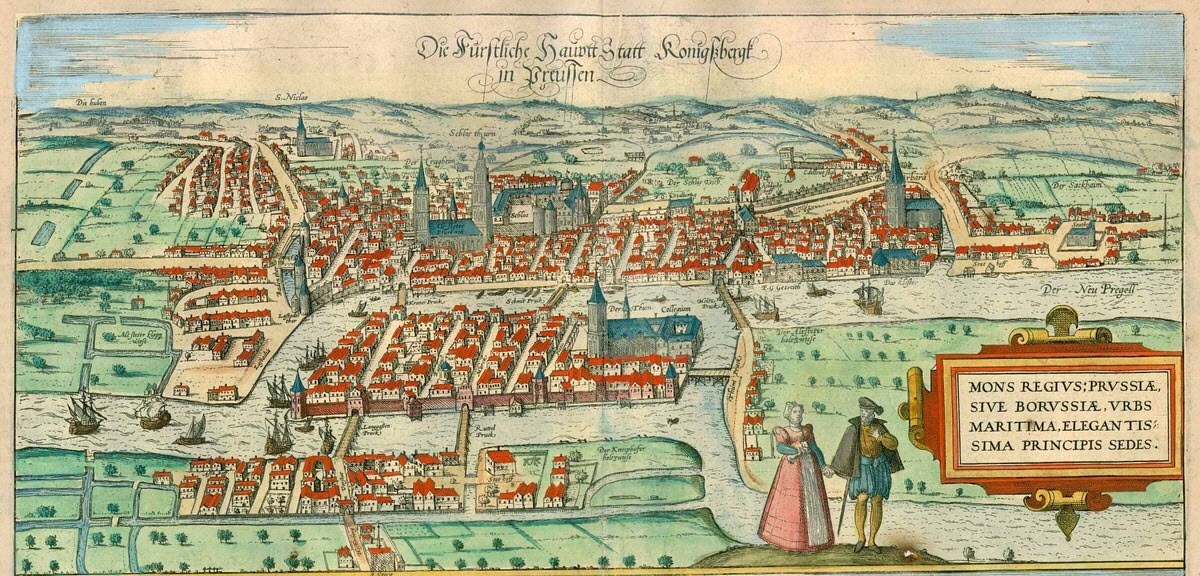
Eulerian circuits are named after Leonhard Euler, who solved in 1736 a famous problem known as the Seven Bridges of Königsberg. The image below shows the city of Königsberg (now Kaliningrad, Russia.) Notice there are 7 bridges separating 4 landmasses. Can we cross all 7 bridges without using the same bridge twice?

Naturally, we will model this problem by constructing a multigraph, whose four vertices correspond to the landmasses, and whose seven edges correspond to the bridges.

The degree sequence is $ 5333 $. The following theorem provides a negative answer to the 7 bridges problem.

Theorem: A connected multigraph $ G $ has an Eulerian circuit if and only if every vertex has even degree.
Similarly, it has an Eulerian trail from $ u $ to $ v $ iff $ u $ and $ v $ are the only odd-degree vertices.

Proof of Necessity:

Suppose $ G $ is a graph containing an Eulerian circuit $ C $. Every time a vertex of $ G $ appears in $ C $, this accounts for an two number of edges (1 in and 1 out). Since $ C $ is a circuit, none of the edges in $ C $ are repeated. Furthermore, since $ C $ is Eulerian, every edge of $ G $ appears in $C $. Finally, since $ G $ is connected, every vertex must appear in $ C $. Altogether, these facts show that every vertex of $ G $ has even degree. A similar argument shows if $G $ has an Eulerian trail from $ u $ to $ v $, then $ \text{deg}(u) $ and $ \text{deg}(v) $ are odd, and all other vertices even.

Proof of Sufficiency:

First, consider the case where $ G $ is a connected graph such that every vertex has even degree. We will prove that $ G $ has an Eulerian circuit using induction on the number of edges $ \# E( G) $.

As a base case, we may assume $ \# E(G) = 0.$ In this case, connectedness implies that $ G $ is a graph with one vertex $ v $, and the sequence $ C = (v) $ is an Eulerian circuit, since there are no edges in $G $ to visit.

Now, suppose $ G $ is a graph with $ \# E(G) > 0$. We establish two claims.

Claim 1: $ G $ contains a circuit.

Proof: Let $ P \subseteq G $ be a path of maximal length, with ends $ u $ and $ v $. Since $ \text{deg}(u) \ge 2 $, $ u $ must have an incident edge $ e=uw \notin E(P) $. However, we cannot have $ w \notin V(P) $, since then we could get a path longer than $ P $. Thus, $ w \in V(P) $, and following $ P $ from $ u $ to $ w $ and then $ e $ gives us a circuit (in fact, a cycle.) (Note: this argument will give you a hint about how to solve Homework 1's Problem 5).

Claim 2: A maximal circuit $ C $ in $ G $ is Eulerian.

Proof: Suppose not, and consider the subgraph $ G' \subseteq G $ obtained by deleting edges in $ C $. If $ C$ was not Eulerian, then $G ' $ would have a connected component $ H $ with at least one edge. Since every vertex in $ H $ has lost an even number of edges from $ C$, we may apply the inductive hypothesis to see that $ H $ has an Eulerian circuit $ D $. The circuits $ C $ and $ D $ are both edge-disjoint. They also have a common vertex $ u \in V(C) \cap V(D) $: this follows from the connectivity of $ G $. Without loss of generality, we may assume that $ u $ is the starting vertex for both circuits; with this assumption, we could then obtain a new Eulerian circuit by gluing, namely $ (C, D) $, whose length is strictly longer than that of $ C $. This is a contraction, so the claim that $ C $ is an Eulerian circuit must hold.

Trail Case:

Suppose now that $ G $ is connected and $ u, v \in V(G) $ are the only vertices of odd degree. Construct a new graph $ G^* $ with $ V(G^*) = V(G) \cup \{w\} $, where $ w $ is a new vertex not already in $ V(G) $, and $ E(G^*) = E(G) \cup \{uw, vw\} $. By our previous arguments, the graph $ G^* $ contains an Eulerian circuit. Finally, we may observe that removing the edges connected to $ w $ from this circuit produces a $ uv$-Eulerian trail in the original graph $ G $.

Hamiltonian Graphs

We have seen that Eulerian graphs have a characterization which can be checked efficiently: examine each vertex and check if it has even degree. In fact, our inductive proof of this characterization already suggests an algorithm for constructing an Eulerian circuit, given that the graph is in fact Eulerian: find a circuit, delete the edges, and recurse on some smaller connected component.

The Seven Bridges Problem that motivated our study of Eulerian graphs is superficially similar to the Traveling Salesperson Problem (TSP), which relates to Hamiltonian graphs, those graphs which contain a cycle through every vertex. Suppose a salesperson must visit $ n $ cities, labeled $ 1, 2, \dots, n $. The cost of traveling from city $ i $ to city $ j $ is given by a nonnegative number $ c (i,j) \ge 0 $. The TSP then asks: what is the minimum cost trip that visits all cities?

Recognizing Hamiltonian graphs is a special case of TSP. To see this, let $ G $ any graph on $ V(G)=\{1, \dots, n\} $. We define a set of $ \binom{n}{2} $ costs as follows: whenever $ 1 \le i < j \le n $, $$ c(i,j) = \begin{cases} 0 & \text{if } ij \in E(G) \\ 1 & \text{if } ij \notin E(G) \end{cases} $$ With this choice of costs, observe that $ G $ has a Hamiltonian path $ \iff $ Salesperson has a free trip. Furthermore, $ G $ has a Hamiltonian $uv $-path if and only if the graph $G^* $ is Hamiltonian, where $ G^* $ constructed by joining $ u$ and $v $ to a new vertex as in our characterization of graphs with Eulerian trails.

As we have already noted, an efficient characterization of Hamiltonian graphs is currently unknown: providing one would be a major breakthrough. On the other hand, it is possible to give some sufficient conditions implying Hamiltonicity.

Ore's Theorem: Let $ G $ be a connected graph with $ \#V(G) \ge 3 $ and such that $ d(u) + d(v) \ge \#V(G) $ whenever $ uv \notin E(G) $. Then $ G $ has a Hamiltonian cycle.

Note that the converse of Ore's theorem is false: there are many Hamiltonian graphs where $ d(u) + d(v) < \# V(G) $ for some non-edge $ uv \notin E(G) $. The simplest example is the cycle $ C_5 $, shown below.

Our proof of Ore's Theorem will rely on the lemma below.

Lemma 1: If $ G $ is connected and non-Hamiltonian, then the length of a longest path in $ G $ is at least the length of a longest cycle.

In contrapositive form, Lemma 1 states that if a longest path in a connected graph $ G $ is shorter than a longest cycle, then $ G $ is Hamiltonian. Indeed, in any Hamiltonian graph $G $ on $ n $ vertices, the longest cycle has length $ n $ and a longest path has $ n- 1 $.

Proof: Let $ C $ be a longest cycle in $ G $. Since we assumed $ G $ is not Hamiltoninan, the cycle has length $ \ell < \#V(G) $. Since $ G $ is connected, there exists some vertex $ v \notin V(C) $. For any $ v_0 \in V(C) $, there exists an $ v_0 $-path $ P = v_0 v_1 \dots v $. Pick the smallest index $ i $ such that $ v_i \notin V(C) $, so that $ v_{i-1} \in V(C) $. We may write our cycle as $ C = (v_{i-1} , u_1, \ldots ,u_{\ell -1 }, v_{i-1} ) $. From this description of $ C $, we may obtain a path of length $ \ell $, namely $ (v_i, v_{i-1} , u_1, \ldots , u_{\ell -1 }) $.

Proof of Ore's Theorem:

Assume $ G $ satisfies the assumptions of Ore's theorem: $ \# V(G) \ge 3 $, and $ d(u) + d(v) \ge \# V(G)$ for any nonedge $uv \in E(G) $. Using the pigeonhole principle as in our "Connectivity Criterion" from Section 2, we obtain that $ G $ that is connected.

Suppose now that $G $ is non-Hamiltonian. Consider a longest path in $ G $, $ P = v_0 \dots v_\ell $. Note that $ \# V(G) \ge 2 $ implies $ \ell \ge 2 $. Having assumed that $ G $ is not Hamiltonian, it follows from Lemma 1 that $ G $ contains no cycle of length greater than $ \ell $. In particular, this implies $ v_0 v_\ell \notin E(G) $.

Consider the sets: $$ A = \{ i \mid 1 \le i \le \ell, \quad v_0 v_i \in E(G) \} $$ $$ B = \{ i \mid 1 \le i \le \ell, \quad v_{i-1} v_\ell \in E(G) \} $$

We make the following two observations:

$ \Gamma(v_0) \cup \Gamma(v_\ell) \subseteq V(P) $ (otherwise, we could get longer path)
$ A \cap B = \emptyset $ (otherwise, could get a cycle of length greater than $ \ell $: to see this, note that if $ i\in A \cap B $, then we could construct the a cycle $ v_0 \dots v_{i-1} v_{\ell} v_{\ell -1} \dots v_i v_0 $, which has length $ \ell + 1$, see below.)

Our assumptions on $ G $ and the two observations above imply that $$ \# V(G) \le d(v_0) + d(v_\ell) = \#A + \#B \le \ell < \ell +1 = \# V(P),$$ which is a contradiction since the path $ P \subset G $ cannot have strictly more vertices than $ G $. Thus, our asumption that $ G $ was non-Hamiltonian cannot hold.

Shortest Paths

Graph Distance: On a connected graph, for $ u, v \in V(G) $, $ d(u,v) $ is the length of a shortest $ uv $ path.

Finding a longest path has played a role in the proofs of several of our results so far. Unfortunately, this is yet another problem that is difficult to solve in practice. Surprisingly, it is much easier to find shortest paths in a graph $ G $. This is true even if we attach nonegative weights/costs to the edges of $G $.

Dijkstra's Algorithm finds a shortest $ s-v $ path for some fixed $ s \in V(G) $, and all $ v \in V(G) \setminus \{s\} $. More generally, this algorithm works for graphs with cost function on edges, $ c: E(G) \to \mathbb{R}_{\ge 0} $. $$ d(u,v) = \displaystyle\min_{P: \text{ a } uv\text{-path}} \Bigg( \displaystyle\sum_{e \in P} c(e)\Bigg)$$

Algorithm: Dijkstra(G, s, c)

Input: Connected graph $ G $, source $ s \in V(G) $, costs $ c $

Output: Shortest path distances $ d(s,v) $ for all $ v \in V(G) $

$ V \leftarrow \{s\} $, $ d(s,s)=0 $ // Initialize set of "visited" vertices and distances

while $ V \neq V(G) $:

Select $ u \in V(G) \setminus V $ and $ v \in V $ that minimize:

$ \text{cost} = d(s,v) + c(v,u) $

update $ V \leftarrow V \cup \{u\} $

$ d(s,u) \leftarrow \text{cost} $

return all distances $ d $

To illustrate Dijkstra's algorithm, let us consider an example of an undirected graph $ G $, with numeric labels indicating the cost $ c(u,v) $ on each edge $ uv \in E(G) $:

We consider each iteration of the "while" loop in Dijkstra's algorithm below.

First iteration

$ V = \{ s \} $
Total costs of cut edges: sa (cost 6), sb (cost 2).

Second iteration

$ V = \{ s , b\} $
Total costs of cut edges: sa (cost 6), bd (cost 2+2=4 ), be (cost 2+5=7).

Third iteration

$ V = \{ s , b, d\} $
Total costs of cut edges: sa (cost 6), da (cost 1+4=5), dc (cost 4+4=8), de (cost 4+2=6), be (cost 2+5=7)

Fourth iteration

$ V = \{ s , b, d, a\} $
Total costs of cut edges: ac (cost 5+2=7), dc (cost 4+4=8), de (cost 4+2=6), be (cost 2+5=7)

Fifth iteration

$ V = \{ s , b, d, a, e\} $
Total costs of cut edges: ac (cost 5+2=7), ec (cost 6+4=10), dc (cost 4+4=8)

Upon termination, all vertices are visited, and Dijkstra's Algorithm has generated a search tree in which every vertex is labeled by its distance from the source.

Theorem: Dijkstra's algorithm finds all shortest paths from $ s $ to all other vertices of $ G $.

Proof: Induction on the number of visited vertices. The base case $ \# V = 1 $ is trivial, so suppose $ \# V > 1 $. Let $ v \in V $ be the most recently visited vertex, and suppose $ uv $ is the corresponding cut edge. By inductive hypothesis, Dijkstra's algorithm has already generated a shortest $ su $-path, which we denote by $ P_u $. Now suppose $ P $ is an arbitrary $ sv $-path. Let $ y \in V(P) $ be the closest non-visited vertex to $ s $, and $ x \in V(P) $ its left-neighbor on $ P $. The update rule in Dijkstra's algorithm then tells us that $$d(s, x) + c(x,y) \ge d(s,u) + c(u,v) .$$ Since all costs along edges are nonngeative, this then implies that the total cost of $ P$ is at least $d(s,u) + c(u,v)$. Thus, the path $ (P_u, uv) $ is a shortest $ sv $-path.

4. Trees

Basic Facts and Examples

Tree Theorem: Let $ G $ be a graph. The following are equivalent:

$ G $ is a tree (connected, acyclic graph).
$ G $ is a maximally acyclic graph (adding any edge creates a cycle).
$ G $ is a minimally connected graph (deleting any edge disconnects the graph).

A tree is any graph satisfying the equivalent conditions of this theorem.

Proof Sketches:

(1) $\Rightarrow$ (2): If $ G $ is connected and acyclic, adding an edge $ uv $ creates a cycle because a path between $ u $ and $ v $ already existed.
(2) $\Rightarrow$ (3): If $ G $ is maximally acyclic, adding $ uv $ creates a cycle, implying a path existed. If we remove an edge, it becomes disconnected (sketched).
(3) $\Rightarrow$ (1): We need to show a minimally connected graph is acyclic. If $ G $ contained a cycle, we could delete an edge from the cycle and $ G $ would remain connected (detour along the rest of the cycle). This contradicts minimality.

Spanning Trees

A subgraph $ H \subseteq G $ is spanning if $ V(H) = V(G) $.
Corollary: Any connected graph $ G $ contains a spanning tree. (Proof: Delete edges from cycles until acyclic but still connected).

Properties of Trees

Let $ T $ be a tree.

$ \#E(T) = \#V(T) - 1 $.
$ T $ contains at least two leaves (vertices of degree 1) for $ n \ge 2 $.

Proof of leaf property: Suppose $ d(v) \ge 2 $ for all $ v $. We could construct a cycle by walking along edges, contradicting that $ T $ is a tree. More formally, if $ v $ was the only leaf: $ 2\#V(T) - 2 = 2\#E(T) = \sum d(u) \ge 1 + 2(\#V(T)-1) $, which leads to a contradiction.

Minimum Spanning Trees (MST) & Kruskal's Algorithm

Problem: Connect cities (vertices) with edges having costs, such that total cost is minimized.
Input: Connected graph $ G $, cost function $ c: E(G) \to \mathbb{R} $.
Goal: Find a spanning tree $ T $ minimizing $ \sum_{e \in E(T)} c(e) $.

Kruskal's algorithm is a "greedy algorithm" for finding a minimum spanning tree.

Algorithm: Kruskal(G, c)

Input: Connected graph $ G $, costs $ c: E(G) \to \mathbb{R} $

Output: A minimum spanning tree $ F $

$ F \leftarrow (V(G), \emptyset) $ // Initialize graph with no edges

Sort edges such that $ c(e_1) \le c(e_2) \le \dots \le c(e_m) $

for $ i = 1 $ to $ m $:

if $ F + e_i $ has no cycles:

$ F \leftarrow F + e_i $

return $ F $

The correctness of Kruskal's algorithm is the content of our next theorem.

Theorem: Kruskal's Algorithm solves the MST problem.

Proof (Exchange Argument): We claim the graph $ F $ is contained in some MST at any stage. Suppose $ F $ is contained in an MST $ T $ and we choose edge $ e $. If $ e \in T $, done. Otherwise, $ T+e $ contains a cycle $ C $. Since $ F+e $ is acyclic, there exists an edge $ e' \in C \setminus F $. Replacing $ e' $ with $ e $ in $ T $ creates a new tree $ T' = T - e' + e $ with cost $ \le $ cost of $ T $. Thus, the greedy choice is valid.